
In this guide
An MIS report in Excel is a monthly management pack that pulls figures out of your accounting ledger (revenue, expenses, cash, receivables and payables) and summarises them on one or two sheets so the owner or management can read performance without opening the books. The reliable way to build one is to keep raw transaction data on a single clean sheet, hold it as an Excel Table, and then aggregate it on a separate output sheet using PivotTables or SUMIFS. This article walks through that method step by step, adds the Indian layer of GST, TDS and cost centres, and is a how-to guide only: if you want the work done for you, our MIS Reporting Services team builds and runs these packs.
What is MIS in MS Excel?
MIS stands for Management Information System. In an Excel context it simply means a structured workbook that turns raw accounting data into decision-ready summaries: monthly revenue by product, cost by department, gross margin, cash position, debtor ageing and a few key ratios. It is not a new set of books. It is a reporting layer that sits on top of your General Ledger and should reconcile to the same Trial Balance your accountant closes each month. If the MIS total does not match the ledger, the MIS is wrong, not the ledger.
The distinction that trips people up is MIS versus advanced Excel. Advanced Excel is a skill set (formulas, pivots, Power Query, charts). MIS is the discipline of deciding what management needs to see and presenting it consistently every month. You can know every Excel function and still build a useless MIS if the report does not answer a real business question. For a fuller treatment of report structure, see our companion piece, What Is an MIS Report? Formats and Examples for Business.
Is Excel an MIS tool?
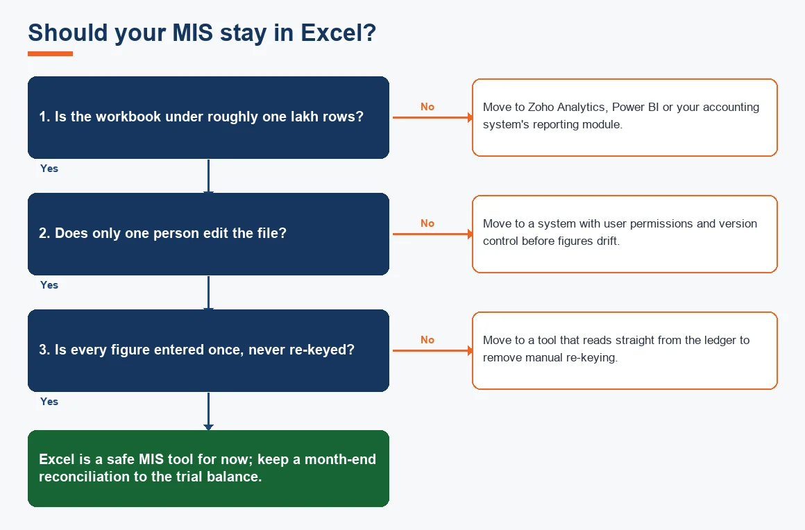
Yes, for a single small business Excel is a perfectly good MIS tool, and for most owner-run firms it is the right first tool. It is cheap, everyone can read it, and it is flexible enough to model any business. What Excel is not is a system of record. It has no edit history, no user permissions and no automatic link back to source vouchers, so it depends entirely on the discipline of whoever maintains it. The moment two people edit the same file, or the same figure is keyed twice, Excel starts to drift from the books silently. That is the line between using Excel well and outgrowing it, and we return to it at the end.
How to create an MIS report in Excel, step by step
The whole method rests on one rule: separate the data from the report. Keep transactions on one sheet and never write a summary formula on it. Do all the aggregation on a second sheet. That single habit is what keeps an MIS file alive month after month instead of breaking.
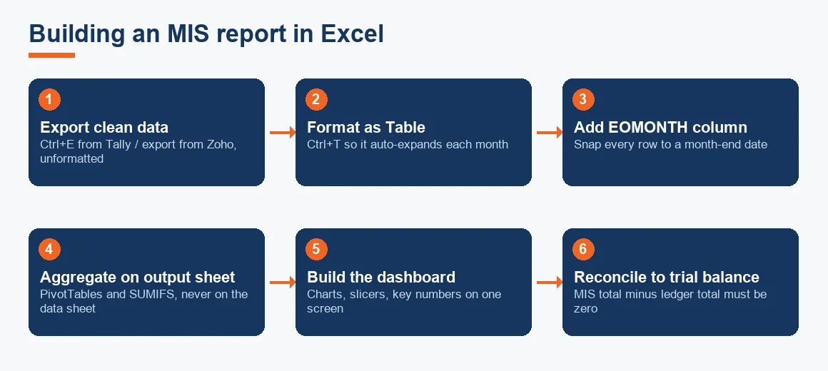
- Export clean data from your accounting software. In TallyPrime, open the Day Book or a monthly Trial Balance and press Ctrl+E to export to Excel or CSV. In Zoho Books or Xero, export the transaction detail or general ledger for the period. Export unformatted: no merged cells, no subtotals, no colour. You want a flat list of rows.
- Lay the data out as a proper table. One row per transaction, one column per attribute: Date, Voucher Type, Ledger, Ledger Group, Cost Centre, GSTIN, State, TDS Section, Debit, Credit, Amount. Select it and press Ctrl+T to convert it to an Excel Table. A Table auto-expands when you paste next month's rows, so every downstream pivot and formula picks up new data on refresh.
- Add an EOMONTH helper column. Put =EOMONTH([@Date],0) in a column called Month End. This snaps every transaction to a single month-end date, which is what you group and total on.
- Build the output sheet. On a separate sheet, create a PivotTable from the Table (Insert then PivotTable). Drag Month End to Rows, Cost Centre or Ledger Group to Columns, and Amount to Values. This is your revenue-and-cost summary.
- Add ratios and variance. Below or beside the pivot, use SUMIFS to pull specific figures (for example total revenue, total direct cost) into a clean summary block, then compute gross margin, growth and budget variance. Wrap each in IFERROR so an empty month prints blank, not an error.
- Reconcile to the trial balance. Add one check cell: MIS revenue minus ledger revenue should be zero. If it is not, fix the data before you circulate anything. Bake this into a Month-End Close Checklist so it happens the same way every month.
How to create an MIS dashboard in Excel
A dashboard is just the output sheet made readable. Once the PivotTables exist, add PivotCharts (a column chart for revenue by month, a bar chart for cost by department, a line for cash trend) and place them on one sheet with the key numbers as large text at the top. Add a slicer on GSTIN, branch or cost centre so a multi-state business can read the same MIS filtered to one location without building a separate file. Keep it to a single screen: management reads a dashboard for ten seconds, not ten minutes. For the metrics worth putting on it, our note on Key Financial KPIs Every MIS Dashboard Should Track is a good starting list, and a ready structure is in Monthly MIS Report Format for Management (Free Template).
What Excel skills help with MIS?
You do not need everything Excel offers. Five functions and one feature carry most Indian MIS work:
- SUMIFS: totals ledger amounts by month, cost centre and group. This is the workhorse of the summary block.
- XLOOKUP (or INDEX with MATCH): pulls the ledger group, GST rate or budget figure from a master sheet into the data.
- IFERROR: hides divide-by-zero and no-data errors so the pack looks clean.
- EOMONTH: aligns every transaction to a month-end column for grouping.
- TEXT: formats month labels and amounts consistently.
- PivotTables and slicers: the aggregation engine and the filter layer.
Power Query is worth learning next: it lets you clean and combine the monthly Tally or Zoho exports automatically, so month two takes minutes instead of an afternoon. Beyond that, more Excel skill adds polish, not reliability.
Worked example: budget versus actual variance
The most useful single view in an MIS is budget against actual, with the variance and its direction called out. Suppose a services firm has these October figures. The variance is Actual minus Budget, and variance percentage is variance divided by Budget. For cost lines, an actual above budget is unfavourable; for revenue, an actual above budget is favourable. All figures in INR.
| Line item | Budget (INR) | Actual (INR) | Variance (INR) | Variance % | Read |
|---|---|---|---|---|---|
| Revenue | 40,00,000 | 44,00,000 | +4,00,000 | +10.0% | Favourable |
| Direct cost | 18,00,000 | 20,70,000 | +2,70,000 | +15.0% | Unfavourable |
| Gross profit | 22,00,000 | 23,30,000 | +1,30,000 | +5.9% | Favourable |
| Overheads | 12,00,000 | 12,60,000 | +60,000 | +5.0% | Unfavourable |
| Net profit | 10,00,000 | 10,70,000 | +70,000 | +7.0% | Favourable |
The story the numbers tell: revenue beat budget by 10 percent, but direct cost rose 15 percent, so gross margin actually slipped from 55.0 percent (22,00,000 on 40,00,000) to 53.0 percent (23,30,000 on 44,00,000). Net profit is up in rupees but the business is earning slightly less on each rupee of sales. That is exactly the kind of signal an MIS exists to surface, and it is invisible in a plain profit figure. A structured Variance Analysis against a Contribution Margin Dashboard turns this into a monthly habit rather than a one-off spot check.
Adding the Indian layer: GST, TDS and cost centres
An MIS built only for management reporting misses easy wins. If your source Table already carries GSTIN, State and TDS Section columns, the same data can drive your statutory reconciliations. Add a pivot that totals input GST by GSTIN and you have a first-pass check against your GSTR-2B Input Tax Credit Matching; the definitive figures still come from the GST portal and CBIC guidance at cbic-gst.gov.in, but the MIS flags gaps early. A TDS Section column lets you total deductions by section, which matters where Section 194Q on purchase of goods applies; the operative rules sit with the Income Tax Department. A Cost Centre column, meanwhile, is what makes department and branch profitability possible at all. Building the ledger cleanly in the first place is where our Backlog Bookkeeping / Catch-Up work pays for itself: an MIS is only as good as the data underneath it.
Receivables and payables belong on the pack too. A debtor ageing pivot, read alongside Days Sales Outstanding (DSO), tells management how much cash is stuck; this is the same discipline our Accounts Receivable Outsourcing and Accounts Payable Outsourcing teams run day to day. Where the MIS also tracks fixed assets, a depreciation schedule feeds the numbers; our Depreciation Calculator works out the Schedule II charge you would drop into the pack.
When should MIS reporting move out of Excel?
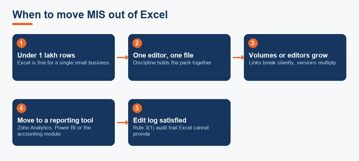
Excel earns its place until three things happen: the workbook passes roughly one lakh rows, more than one person edits it, or the same figures get keyed twice. Past that point, links break silently, versions multiply, and no edit history survives to show who changed what. At that stage a reporting tool (Zoho Analytics, Power BI, or the reporting module of your accounting system) takes over, reading straight from the ledger with no manual re-keying. There is also a compliance angle: Rule 3(1) of the Companies (Accounts) Rules requires an edit log in the books of account, and a spreadsheet cannot provide one; the rule text is on the MCA site. Use the decision below to judge where you stand.
Key terms
- General Ledger: the master record of all accounting transactions that an MIS summarises.
- Trial Balance: the closing list of ledger balances your MIS must reconcile to each month.
- Variance Analysis: comparing actual figures to budget and explaining the gap.
- Days Sales Outstanding (DSO): average days to collect receivables, a core MIS cash metric.
- Month-End Close Checklist: the repeatable steps that make each month's pack consistent and reconciled.
Key takeaways
- Separate raw data from the report: one clean Excel Table, one output sheet. This single habit keeps the file alive.
- SUMIFS, XLOOKUP, IFERROR, EOMONTH and PivotTables cover most Indian MIS work; Power Query is the next skill worth learning.
- Every pack must reconcile to the trial balance, or it becomes a parallel truth that drifts from the books.
- Carry GSTIN, State, TDS Section and Cost Centre on the source Table so the same data also drives GST and TDS checks.
- Leave Excel once you pass about one lakh rows, more than one editor, or double keying: Rule 3(1) of the Companies (Accounts) Rules needs an edit log Excel cannot give.
The pattern in this article is the same one professional teams use; the only real variable is discipline. If maintaining it every month is not the best use of your time, that is the point at which our MIS Reporting Services take over the pack. For how an MIS differs from your statutory accounts, read MIS Report vs Financial Statements: What's the Difference?
Decision guide